For this tutorial series, we will be using the genlight object that we created in the previous tutorial. Original data in HapMap format used in TASSEL was converted to genlight object. Here b will be our genlight object that we previously created in Tutorial P01.
Import library
library(LDcorSV)
library(adegenet)
library(ggplot2)
library(scales)
library(tidyverse)
library(dpaudelR)
Find clusters
grp <- find.clusters(b, max.n.clust=20) # choose PCs to retain=25, and cluster=3
Get BIC values
head(grp$Kstat, 10)
    grp$Kstat
K=1  199.4066
K=2  198.5858
K=3  198.9646
K=4  200.5819
K=5  202.1871
K=6  203.6212
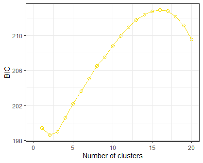
Plot BIC vs number of clusters
bicgrp <- as.data.frame(grp$Kstat)
bicgrp$cluster <- row.names(bicgrp)
bicgrp$NumCluster <- as.numeric(str_replace_all(bicgrp$cluster, 'K=',''))

# Actual plot
bicgrp %>% ggplot(aes(x=NumCluster, y=`grp$Kstat`))+
  geom_point(cex=2, shape=1)+
  geom_line()+
  xlim(0,20)+
  ylab('BIC')+
  xlab('Number of clusters')+
  theme_bw()